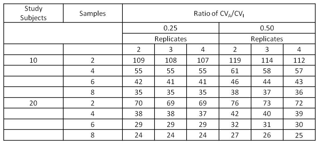
Biological variation studies can be performed with moderate number of subjects since increasing the number of occasions samples are taken and increasing the number of replicates of each assessment (i.e., duplicate, triplicate or more) reduces the confidence interval of the within-subject standard deviation and, therefore, increases the power of the study.¹ That said, a minimum of 10 subjects is recommended (but power increases with more subjects) for testing on at least six occasions (usually weekly) with samples run, at least, in duplicate. The ‘ideal’ minimum number of subjects has been shown to depend on the ratio of standard deviation of within patient variation to standard deviation of analyzer variation. The following table shows that the width of the 95% confidence interval (CI) for various number of individuals, samples and replicates when the ratio of CV_A/CV_I is 0.25 and 0.5. For example, for a measurand with CV_A/CV_I =0.25, 6 collections, the width of the CI reduces from 42 to 29% of the expected within patient standard deviation when increasing from 10 to 20 study subjects; further reductions of the confidence interval from running intriplicate or extending to 8 samples are modest.¹

Table 1: Width of 95% Confidence Intervals for Within Subject Biologic Variation (SDI) for varying numbers of subjections, samples, replicates for ratios of CV_A/CV_I of 0.25 and 0.50 (adapted from Røraas et a 2012)¹

‘Guesstimates’ of the ratio of standard deviation of within patient variation to standard deviation of analyzer variation can be made by looking at studies of other species for similar analytes. For example, the liver enzymes, ALP, ALT and AST all had within patient coefficient of variation (CV_I) of 12.5% to 15% for a recent study of cats² and 13% to 20% for a recent study of dogs;³ the analytical coefficient of variation (CV_A) or precision can be determined by recent QC from the analyzer to be used in the study. The precision in the aforementioned studies was ~4-5% for the cat study² and 6-9% for the dog study.³ This gives ratios in the order of 0.3 to 0.5.

Outliers should be assessed for each analyte using a test such as Tukey’s outlier identification method and assessed for each measurand on three levels: across the entire group of subjects, for each subject individually and for individual subjects with outlying variability compared with the other subjects in the group.

There are no specific guidelines for how to treat outliers. Common sense with an emphasis on retaining data is important and can be helped by assessment of normality of the distribution of the residuals (see below) e.g., considerable variation between duplicate samples from the same patient from the same day indicates systematic error and does not contribute data about biological variation.

“A single extraordinary observation, resulting from an analytical blunder in the assay, or a misidentification of the specimen, can exert a profound effect on summary statistics, especially variances. A distinction should be made between an aberrant observation, due to a mistake or accident in the analytical procedure, and an outlier. In some cases, the outlier is known to be aberrant, but more often no explanation can be found for an unusual value.”⁴

Routine analysis of variance ANOVA should be used for balanced designs or restricted maximum likelihood (REML) (for balanced and unbalanced designs) should be used to estimate variance components by specifying measurands as outcome variables, subject identification and day (nested within subject identification) as random effects. Most statistical software packages have these models; seeking advice from those with experience running these models is important as this is one of the most crucial aspects of running biological variation studies.

The normality of residuals for ANOVA or REML should be evaluated by visual inspection of histograms and normal plots of residuals; using goodness-of-fit/omnibus tests such as the Shapiro-Wilk or Darling-Anderson may be used to help assess the normality. An assessment of maintaining or excluding potential outliers can be made by assessing the distribution of residuals. A normal distribution indicates that outliers are not affecting the variance components. If the distribution is not normal, an assessment needs to be made if this due to outliers that should be excluded or results from normal/healthy subjects; typically, if the distribution is skewed due to results from normal/healthy subjects, there will be more results causing the skew than if the skew is due to outliers.

When the distribution is normal, inter-individual or group variation (CV_G), intra-individual variation (CV_I) and the variation occurring between duplicates, or analytical variation (CV_A) can then be calculated from the variance components (by dividing by the relevant mean). These should be reported with 95% confidence intervals. CIs in nested ANOVA designs can be determined within the statistical programming environment ‘R’ (http://www.r-project.org/), using the‘varcompci’ package.⁴ From these, the Index of Individuality (II) can be calculated as:

II = CV_G /√( CV_A² + CV_I²)

The use of CV_G as the numerator results in higher values for increased intra-individual variation.^{2-4, 6} With the traditional use of CVG as the denominator, indices of individuality <0.6 data-preserve-html-node="true" indicate that subject-based reference values are more appropriate (and population-basedse of CVG asreference intervals are of limited utility) and indices >1.4 indicate population-based reference intervals are more appropriate. With the more intuitive inverse formula (CV_G as the numerator) indices of individuality >1.67 indicate that subject-based reference values are more appropriate and indices <0.7 data-preserve-html-node="true" indicate population-based reference intervals are more appropriate.

Reference change values (RCVs) can be calculated for 95% confidence intervals in percentage terms according to:

RCV = Z x √2x √( CV_A² +CV_I² )

Undirectional (Z = 1.65) or bidirectional (Z = 1.96) results should be calculated depending on whether the measurand is likely to require interpretation when concentrations are either high or low (one-sided or unidirectional) or for both high or low concentrations (two-sided or bidirectional ).

For those analytes where results are not normally distributed, data should be log-transformed (to base e) and then assessed in the same way as for the raw data, using residual diagnostics. CVs should then be back transformed by CV = √(exp σ² –1), as previously described.^7-8 The RCV can then be calculated using the lognormal approach described by Fokkema et al.⁷ Briefly, the ‘lognormal’ standard deviation is calculated from the untransformed CV such that σ = √log (CV² + 1) for each of CV_I and CV_A; then, RCV is calculated as exp(+Z. √ [2. (σ_I² + σ_A²)] for increasing values and as exp(–Z. √ [2. (σ_I² + σ_A²] for decreasing values, where Z = 1.65 when one-sided analysis is appropriate (interpretation of results only concerned with increased or decreased results) and Z = 1.96 for two-sided analysis (both increased and decreased results of significance), and, accordingly, these RCVs are not symmetrical. An example for creatine kinase (CK) in cats² is shown below. The ‘raw’ results (Figure 1) show that approximately 60% of results (i.e., most cats’ results over the duration of the study) did not show much variation but any variation was more likely to be an increase hence the uneven distribution of results. The assessment of residuals of the log of the results (Figure 2) shows an essentially normal distribution. The calculated RCV was 361% for increases and 34% for decreases which means that an increase in an individual’s serial results need to approach a four times change to be clinically significant but a subsequent 34% decrease is a clinically significant reduction towards normal. If a healthy cat has CK of 500 U/L, the CK may rise to a clinically significant level of 2,000 U/L (four times) when the cat has toxoplasmosis, a reduction back to 1,200 U/L (reduced by 40% of 2000U/L) shows clinically significant improvement.

Adequate precision should be assessed by CV_A < 0.5 CV_I for each measurand.⁹ CV_A < 0.5 . √( CV_I² + CV_G²) should be assessed for each measurand as an indicator of whether analytical variation is sufficient to affect judgment of biological variation, individuality and therefore RCVs.^9-10

References:

1. Røraas T, Petersen PH, Sandberg S. CIs and power calculations for within-person biological variation: effect of analytical imprecision, number of replicates, number of samples, and number of individuals. Clin. Chem. 2012: 1877-1881.
2. Baral RM, Dhand NK, Freeman KP, Krockenberger MB, Govendir M. Biological variation and reference change values of feline plasma biochemistry analytes. J. Feline Med. Surg. 2014;16(4):317-325.
3. Ruaux CG, Carney PC, Suchodolski JS, Steiner JM. Estimates of biological variation in routinely measured biochemical analytes in clinically healthy dogs. Vet. Clin. Path. 2012; 41(4):541-547.
4. Fraser CG, Harris EK. Generation and application of data on biological variation in clinical chemistry. Crit. Rev. Clin. Lab. Sci. 1989;27(5): 409.
5. Civit S, Vilardell M, Hess A, et al. Package ‘varcompci’. Food Control. 2013; 12: 119-125.
6. Walton RM. Subject-based reference values: biological variation, individuality, and reference change values. Vet. Clin. Path. 2012;41(2):175-181.
7. Fokkema MR, Herrmann Z, Muskiet FA, Moecks J. Reference change values for brain natriuretic peptides revisited. Clin. Chem. 2006;52(8):1602-1603.
8. Elassaiss-Schaap J, Heisterkamp SH. Variability as constant coefficient of variation: Can we right two decades in error? Annual Meeting of the Population Approach Group in Europe. St Petersburg, Russia 2009.
9. Cotlove E, Harris EK, Williams GZ. Biological and analytic components of variation in long-term studies of serum constituents in normal subjects. III. Physiological and medical implications. Clin. Chem. Dec 1970;16(12): 1028-1032.
10. Petersen PH, Fraser CG, Jorgensen L, et al. Combination of analytical quality specifications based on biological within-and between-subject variation. Ann. Clin. Biochem. 2002; 39(6):543-550.